Data engineering / Comparison
Streaming vs Batch: Choosing with a Latency Budget Instead of a Trend
Choose between streaming, micro-batch, and batch by deriving a latency budget from the consumer decision, not by following tooling trends.
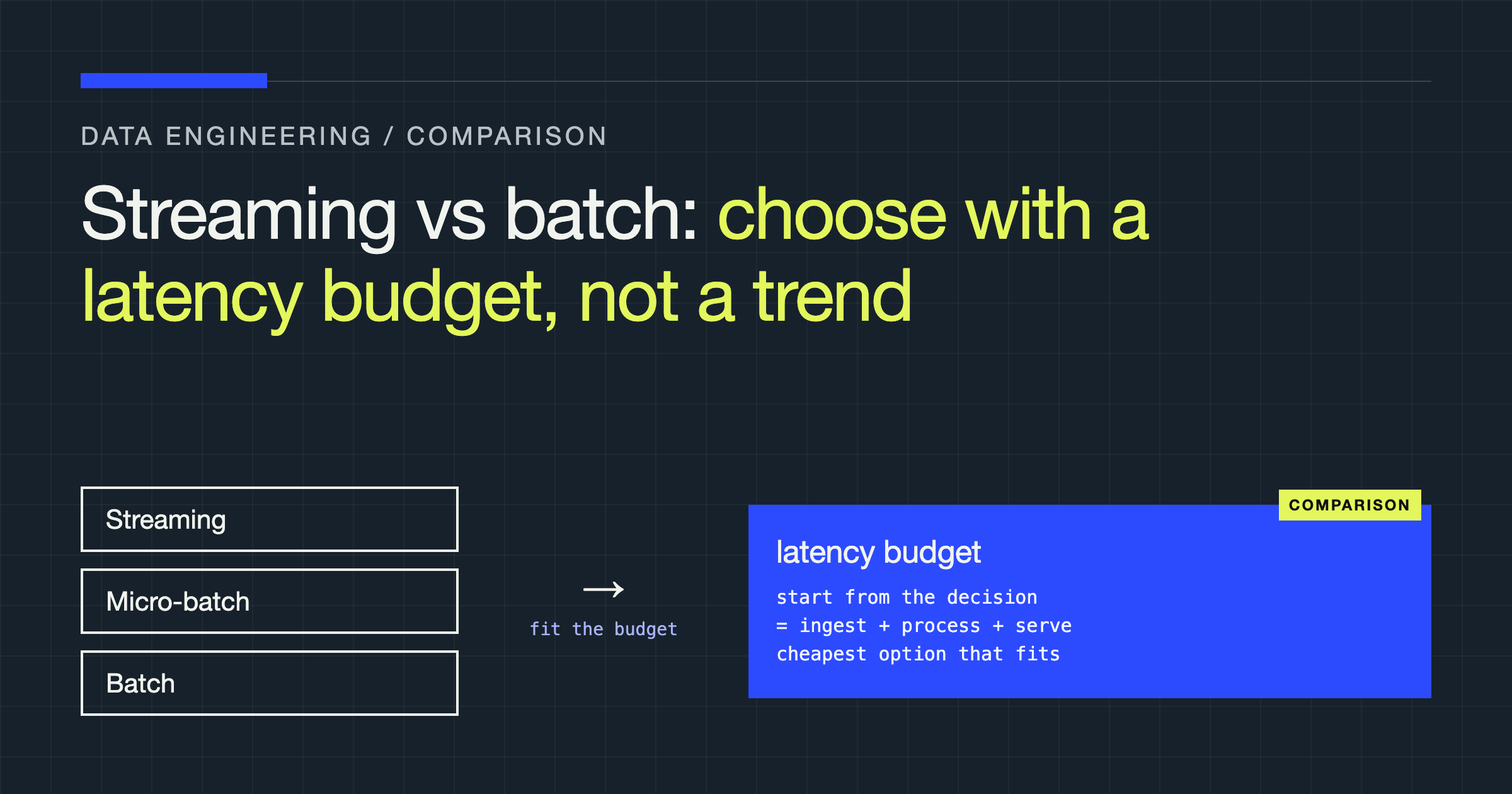
You will decide, by the end of this article, whether your pipeline should run continuously, on a short interval, or on a schedule — from a number you can defend: the latency budget imposed by the consumer of the data. Not from which engine is fashionable, and not from assuming fresher is always better.
Start with the decision, not the engine
Every pipeline supports a decision: a dashboard someone reads, a model that scores a request, an alert that fires, or a system that acts on a row. Three properties of that decision should determine your architecture before you compare tools.
First, freshness requirement: how old can the event be when the decision is made before the decision gets worse? A fraud block arriving after a transaction has settled is not slightly late; it is a weaker decision. A daily reconciliation report does not improve because its input arrived a little earlier.
Second, decision cadence: how often is the decision actually taken? If a team reviews a metric in a morning meeting, data refreshed continuously overnight sat idle for most of that interval. If a system evaluates every arriving request, scheduled processing inserts a wait no downstream optimisation can remove.
Third, staleness tolerance: can the consumer act on a partial picture and revise later, or must it wait for completeness because acting twice, or retracting an action, costs more than waiting?
Together, these give you a total latency budget: the maximum acceptable time between an event at the source and a correct, queryable result reflecting it. Every later choice spends, or wastes, that budget.
Decompose the end-to-end latency
A common mistake is to compare engines by processing speed and ignore the rest of the path. End-to-end latency is a sum, and processing is only one term:
- Ingest: time for the event to leave the source and become available to your processor. Change data capture, polling, and producer batching add delay before your code runs.
- Processing: time to parse, validate, join, aggregate, and transform — the term benchmarks usually measure, and often not the largest.
- Storage commit: time to write the result durably and visibly. Transaction commits, file finalisation, compaction, and index updates can quietly dominate.
- Query and serve: time for the consumer to see the new state. A committed result that a dashboard caches has not arrived yet from the consumer’s point of view.
# Illustrative structure — fill from your consumer's needs
consumer: "the decision, and who or what makes it"
freshness_requirement: "maximum acceptable data age"
decision_cadence: "how often the decision is taken"
staleness_tolerance: "partial data, or wait for completeness"
budget: { ingest: "", processing: "", storage_commit: "", query_serve: "" }
late_data_policy: "revise, side path, or drop after cutoff"
Event time, processing time, and late data
Batch sidesteps a hard problem by waiting: by the time a scheduled job runs, most data for a period has arrived, and the job processes a settled set. Streaming cannot sidestep it: you must decide what a timestamp means while data is still arriving.
Event time is when something happened at the source. Processing time is when your system observes it. They diverge through network delays, offline devices, retries, upstream queues, and clock differences. Any windowed aggregation — totals per interval, sessions, rolling counts — changes meaning depending on which clock you use. Windowing on processing time is simpler and faster, but the windows then describe your arrival pattern, not the real-world sequence you probably care about.
Watermarks manage this in streaming systems: a statement, derived from observed event times, that the stream is believed complete up to a point in event time. When the watermark passes a window’s end, the system can emit the result and release its state. An aggressive watermark is sooner but classifies more arrivals as late; a conservative one is more complete but spends latency waiting for stragglers.
Late data forces a policy, and every policy trades something away. Accept and update, and your consumer must handle revisions — which many dashboards and downstream contracts cannot do. Route late events to a side path, and completeness survives but someone owns reconciliation. Drop after a cutoff, and you protect latency at the price of bounded incompleteness you must measure and surface. Batch postpones this problem, and a rerun quietly absorbs late arrivals — a genuine advantage.
Delivery guarantees, state, and checkpointing
Delivery semantics decide how much correctness work your code must do. With at-least-once delivery, a failure can cause the same event to be processed again, so sinks and updates must be idempotent: applying an event twice must equal applying it once. That means deterministic keys, upserts instead of appends, and deduplication you design, test, and maintain.
Exactly-once processing removes some of that burden, at a cost. Coordinating a state update and an output commit so they succeed or fail together requires transactional machinery and sink support, and adds latency and constraints. The guarantee only holds end to end if the destination can participate in the transaction — whatever the engine promises internally.
State is the second cost centre. Streaming computations that join, deduplicate, or maintain windows hold state for as long as the logic requires. Large state means heavier checkpointing — the periodic durable snapshot used for recovery — and slower recovery from a restore. Checkpointing competes with processing for I/O and CPU, and an unreliable checkpoint becomes a failure mode of its own. Batch jobs hold little long-lived state, and failure usually means rerunning a bounded unit of work.
Backpressure, replay, and backfill
When producers outpace consumers, something has to give. Streaming systems handle this as backpressure: a slow operator signals upstream, queues fill toward their limits, and latency climbs while the system stays correct. Design for it explicitly: decide where buffering lives, how much you tolerate, and what you shed, sample, or spill when the buffer is exhausted. A system with no backpressure plan discovers its overload behaviour in production.
Replay exposes the sharpest asymmetry between the models. Reprocessing a period in batch is ordinary work: point the same job at retained input, write corrected output, and compare. The input was kept precisely so this is possible.
Replaying a stream is painful by comparison. You must re-consume from a retained log within its retention window, reconstruct or reset long-lived state, reconcile side effects already emitted, and replay without corrupting the live result. Backfilling a new streaming job is harder still: it must consume historical volume faster than live traffic arrives, share resources with that traffic, then cut over cleanly. If your domain expects frequent corrections or restatements, that argues strongly for batch, or for a batch path alongside the stream.
Schema change and the operational bill
Schemas change in both models; the blast radius differs. A batch job reads a dataset at a point in time, so a breaking change fails a run: you fix the job or the data and rerun. The failure is loud and bounded.
A streaming job consumes change continuously. An incompatible field type, a renamed column, or a new event variant arrives mid-stream and becomes a poison event: a record the job cannot process, blocking progress if the system retries it indefinitely. You need a route for such records — a dead-letter destination, quarantine with alerting, and a way to resume without losing events queued behind the bad one.
Price in the on-call reality. A failed batch pipeline usually waits for you; the next run, or a rerun, recovers it, and the consumer sees staleness rather than corruption. A stalled streaming pipeline degrades freshness immediately, often under the highest load, because load and failure are correlated. Continuous systems need continuous observability — lag, watermark progress, checkpoint health, state size, per-operator throughput — each alert with an owner who knows what action it implies. If your team cannot staff that attention, that is a design constraint, not a character flaw.
Where micro-batch fits
Micro-batch processes data in small, frequent, bounded sets: a job triggered on a short interval over just the newly arrived data. It reuses the batch model’s strengths — bounded work, simpler recovery, straightforward replay of one interval, familiar tooling — while shrinking the waiting time that dominates batch latency. For many analytical consumers, that lands inside the budget at far less operational complexity than continuous processing.
Its costs are different, not absent. Very small intervals create many tiny files or transactions, pressuring storage and commit overhead, and startup costs repeat constantly. Event-time logic still needs a late-data policy; running more often does not make late data arrive earlier.
# Apache Spark Structured Streaming — trigger interval as latency dial
query = (
    cleaned.writeStream
    .format("delta")
    .option("checkpointLocation", "/checkpoints/orders")
    .trigger(processingTime="2 minutes")  # illustrative interval
    .start()
)
Set that interval by subtracting ingest, commit, and serving costs from the budget. If the remainder exceeds a workable interval, micro-batch is a serious candidate, not a compromise.
Lambda, kappa, and keeping two truths
Lambda architecture pairs a batch layer, producing complete and corrected results, with a speed layer producing fast, approximate results, merged at serving time. You get low latency and eventual correctness, at the price of implementing the same logic twice, in two models, and keeping both in agreement indefinitely.
Kappa architecture makes everything a stream, expressing batch work as replaying the stream with a revised computation. Logic lives in one place — a real simplification — but retention, replay, and state reconstruction must carry the full weight of historical correction, exactly what streaming makes hardest.
Neither is a default. Lambda earns its duplication only when consumers need both immediacy and restated correctness; kappa earns its replay burden only when retention and replay tooling are first-class features. Often, micro-batch, or batch plus one streaming path, serves the requirement with less architecture.
Failure modes worth designing for
Thundering reprocessing occurs when a failure, fix, or backfill recomputes many partitions at once, overwhelming shared storage, downstream sinks, or the recovering system itself. Bound it: reprocess in slices, rate-limit backfills, and separate replay resources from live traffic.
Poison events block streams, as covered above; in batch, one malformed record can fail a run repeatedly until someone intervenes. Quarantine bad records with context to fix them, and make skipping one an explicit, logged decision.
Clock skew corrupts quietly. Incorrect source clocks produce event times in the future or distant past, distorting windows and watermarks in streaming, and landing data in wrong partitions in batch. Monitor the gap between event and arrival time, alert on outliers, and decide in advance whether skewed events are corrected, clamped, or rejected.
Streaming, micro-batch, and batch side by side
| Dimension | Streaming | Micro-batch | Batch |
|---|---|---|---|
| Latency floor | Ingest and commit; potentially very low | Trigger interval plus commit | Schedule plus run time |
| Decision fit | Continuous, per-event decisions | Frequent checks | Periodic decisions and reports |
| Late data | Watermark policy; revisions or drops | Per interval; later intervals correct | Absorbed by rerunning the period |
| Correctness cost | Idempotency or transactional exactly-once | Per-interval idempotency, simpler | Rerun replaces output; simplest |
| State and recovery | Long-lived state; checkpoint, restore | Bounded per interval | Dataset state; rerun bounded job |
| Replay and backfill | Painful; side effects to reconcile | One interval at a time | Straightforward over retained input |
| Schema change | Mid-stream; poison-event handling | Fails an interval; fix, rerun | Fails a run; fix, rerun |
| Cost shape | Always-on compute, paid while idle | Frequent small runs; interval overhead | Scheduled compute, paid while running |
| Operational burden | Continuous monitoring, urgent on-call | Moderate; failures show as staleness | Lowest; failures wait for a rerun |
Verdict: choose from the budget down
Derive the budget first. Write down the decision, its cadence, its freshness requirement, and its tolerance for incomplete data, then subtract ingest, commit, and serving costs. The remainder — time you can spend processing and waiting — selects the model more reliably than any feature comparison.
Choose batch when the remainder fits a schedule, when correctness and restatement matter more than immediacy, and when your team’s attention is finite. It is the simplest model to operate, the easiest to replay, and the most forgiving of failure.
Choose micro-batch when the remainder is too small for a conventional schedule but large enough for a short interval. For many dashboards and near-term analytics, it delivers usable freshness without the continuous system’s state, checkpointing, and on-call costs.
Choose streaming when the decision itself is continuous or per-event, when waiting for an interval would consume the budget entirely, and when you are prepared to pay permanently for late-data policy, idempotent or transactional sinks, state and checkpoint management, poison-event handling, and monitoring someone responds to. That is the price of admission, and a genuine latency requirement makes it worth paying.
The trend will change again. Your consumer’s decision will not. Budget from the decision, and the architecture follows.